Getting Started with wbstats A World Bank R Package

Jan 8, 2018 19 min read R, wbstats

The World Bank is a tremendous source of global socio-economic data; spanning several decades and dozens of topics, it has the potential to shed light on numerous global issues. The wbstats R package provides access to this data.

This post is meant to serve as a reference for getting started with using wbstats. There are lots of things that aren’t mentioned, particularly several of the wb arguments that can be changed. For a more detailed overview see the Github READ ME or Introduction to the wbstats R-package Vignette

You can install:

The latest release version (0.2) from CRAN with

install.packages("wbstats")

The latest development version from github with

devtools::install_github("GIST-ORNL/wbstats")

wbstats version 0.2 includes

Uses version 2 of the World Bank API that provides access to more indicators and metadata than the previous API version
Access to all annual, quarterly, and monthly data available in the API
Support for searching and downloading data in multiple languages
Access to the World Bank Data Catalog Metadata, providing among other information; update schedules and supported languages
Ability to return POSIXct dates for easy integration into plotting and time-series analysis techniques
Returns data in either long (default) or wide format for direct integration with packages like ggplot2 and dplyr
Support for Most Recent Value queries
Support for grep style searching for data descriptions and names
Ability to download data not only by country, but by aggregates as well, such as High Income or South Asia
Ability to specify countries_only or aggregates when querying data

Downloading data with `wb`

The wb function is how you request data from the API. The only thing you need to get started is which indicator(s) you want to download and for what time period. The indicator parameter takes a vector of indicatorIDs that correspond to the data you want to download. We’ll mention how to find these IDs below

library(wbstats)

# Population growth (annual %)
pop_data <- wb(indicator = "SP.POP.GROW", startdate = 2005, enddate = 2016)

head(pop_data)

##   iso3c date    value indicatorID                    indicator iso2c
## 1   ARB 2016 2.045601 SP.POP.GROW Population growth (annual %)    1A
## 2   ARB 2015 2.118210 SP.POP.GROW Population growth (annual %)    1A
## 3   ARB 2014 2.185197 SP.POP.GROW Population growth (annual %)    1A
## 4   ARB 2013 2.248844 SP.POP.GROW Population growth (annual %)    1A
## 5   ARB 2012 2.305073 SP.POP.GROW Population growth (annual %)    1A
## 6   ARB 2011 2.352527 SP.POP.GROW Population growth (annual %)    1A
##      country
## 1 Arab World
## 2 Arab World
## 3 Arab World
## 4 Arab World
## 5 Arab World
## 6 Arab World

Notice that the first “country” listed is Arab World which of course is not a country at all. The default value for the country parameter is a special value of all which as you might expect, returns data on the selected indicator for every available country or region. If you are interested in only some subset of countries or regions you can pass along the specific codes to the country parameter.

The country and region codes that can be passed to the country parameter correspond to the coded values from the iso2c, iso3c, regionID, adminID, and incomeID from the countries data frame in wb_cachelist or the return of wbcache() (more on that later). Any values from the above columns can mixed together and passed to the same call. You can also use the special value country = "countries_only" to return only values for actual countries

# Population growth (annual %)
pop_data <- wb(country = "countries_only", indicator = "SP.POP.GROW", startdate = 2005, enddate = 2016)

head(pop_data)

##   iso3c date     value indicatorID                    indicator iso2c
## 1   ABW 2016 0.4599292 SP.POP.GROW Population growth (annual %)    AW
## 2   ABW 2015 0.5246582 SP.POP.GROW Population growth (annual %)    AW
## 3   ABW 2014 0.5874924 SP.POP.GROW Population growth (annual %)    AW
## 4   ABW 2013 0.5929140 SP.POP.GROW Population growth (annual %)    AW
## 5   ABW 2012 0.5121450 SP.POP.GROW Population growth (annual %)    AW
## 6   ABW 2011 0.3769848 SP.POP.GROW Population growth (annual %)    AW
##   country
## 1   Aruba
## 2   Aruba
## 3   Aruba
## 4   Aruba
## 5   Aruba
## 6   Aruba

To query indvidiual countries you can use their iso2c or iso3c codes.

# Population growth (annual %)
pop_data <- wb(country = "US", indicator = "SP.POP.GROW", startdate = 2005, enddate = 2016)

head(pop_data)

##   iso3c date     value indicatorID                    indicator iso2c
## 1   USA 2016 0.6928013 SP.POP.GROW Population growth (annual %)    US
## 2   USA 2015 0.7297320 SP.POP.GROW Population growth (annual %)    US
## 3   USA 2014 0.7431243 SP.POP.GROW Population growth (annual %)    US
## 4   USA 2013 0.7002623 SP.POP.GROW Population growth (annual %)    US
## 5   USA 2012 0.7464199 SP.POP.GROW Population growth (annual %)    US
## 6   USA 2011 0.7456144 SP.POP.GROW Population growth (annual %)    US
##         country
## 1 United States
## 2 United States
## 3 United States
## 4 United States
## 5 United States
## 6 United States

Queries with multiple indicators return the data in a long data format by default

pop_gdp_long <- wb(country = c("US", "NO"), indicator = c("SP.POP.GROW", "NY.GDP.MKTP.CD"),
                   startdate = 1971, enddate = 1971)

head(pop_gdp_long)

##   iso3c date        value    indicatorID                    indicator
## 1   NOR 1971 7.012934e-01    SP.POP.GROW Population growth (annual %)
## 2   USA 1971 1.264334e+00    SP.POP.GROW Population growth (annual %)
## 3   NOR 1971 1.458311e+10 NY.GDP.MKTP.CD            GDP (current US$)
## 4   USA 1971 1.167770e+12 NY.GDP.MKTP.CD            GDP (current US$)
##   iso2c       country
## 1    NO        Norway
## 2    US United States
## 3    NO        Norway
## 4    US United States

or a wide format if parameter return_wide = TRUE. Note that to necessitate a this transformation the indicator column is dropped.

pop_gdp_wide <- wb(country = c("US", "NO"), indicator = c("SP.POP.GROW", "NY.GDP.MKTP.CD"),
                   startdate = 1971, enddate = 1971, return_wide = TRUE)

head(pop_gdp_wide)

##   iso3c date iso2c       country NY.GDP.MKTP.CD SP.POP.GROW
## 1   NOR 1971    NO        Norway   1.458311e+10   0.7012934
## 2   USA 1971    US United States   1.167770e+12   1.2643337

Search available data with `wbsearch`

wbsearch allows you to search for indicators that match a certain term. By default it searches for matching terms in both the name and description of the indicators.

pop_vars <- wbsearch("Population Growth")

head(pop_vars)

##              indicatorID                          indicator
## 4368         SP.URB.GROW Urban population growth (annual %)
## 4382      SP.RUR.TOTL.ZG Rural population growth (annual %)
## 4415         SP.POP.GROW       Population growth (annual %)
## 8825 IN.EC.POP.GRWTHRAT.   Decadal Growth of Population (%)

From here you can select which indicators we want and pass their indicatorID into the wb function

pop_vars <- wbsearch("Population Growth")

pop_var_ids <- pop_vars[1:3, "indicatorID"]


pop_data <- wb(country = "countries_only", indicator = pop_var_ids, startdate = 2005, enddate = 2016)

head(pop_data)

##   iso3c date       value indicatorID                          indicator
## 1   ABW 2016 -0.08080622 SP.URB.GROW Urban population growth (annual %)
## 2   ABW 2015 -0.07843500 SP.URB.GROW Urban population growth (annual %)
## 3   ABW 2014 -0.07606930 SP.URB.GROW Urban population growth (annual %)
## 4   ABW 2013 -0.13355748 SP.URB.GROW Urban population growth (annual %)
## 5   ABW 2012 -0.27346595 SP.URB.GROW Urban population growth (annual %)
## 6   ABW 2011 -0.46478167 SP.URB.GROW Urban population growth (annual %)
##   iso2c country
## 1    AW   Aruba
## 2    AW   Aruba
## 3    AW   Aruba
## 4    AW   Aruba
## 5    AW   Aruba
## 6    AW   Aruba

That is pretty much all you need to know to get started searching and downloading data. There are of course more things that can be done, but before we do that now is a good time to introduce out friend wb_cachelist

One list to rule them all `wb_cachelist`

For performance and ease of use, a cached version of useful information from the World Bank API is provided with the wbstats R-package. This data is called wb_cachelist and provides a snapshot of available countries, indicators, and other relevant information. wb_cachelist is by default the the source from which wbsearch() searches and the place wb() uses to do input sanity checks. The structure of wb_cachelist is as follows

library(wbstats)

str(wb_cachelist, max.level = 1)

## List of 7
##  $ countries  :'data.frame': 304 obs. of  18 variables:
##  $ indicators :'data.frame': 16978 obs. of  7 variables:
##  $ sources    :'data.frame': 43 obs. of  8 variables:
##  $ datacatalog:'data.frame': 238 obs. of  29 variables:
##  $ topics     :'data.frame': 21 obs. of  3 variables:
##  $ income     :'data.frame': 7 obs. of  3 variables:
##  $ lending    :'data.frame': 4 obs. of  3 variables:

Inside the wb_cachelist is a data.frame for every major endpoint of the World Bank data API. Some of them such as lending and income are not as interesting as others, but for our purposes here we’ll quickly highlight the countries and indicators data.frames.

The `countries` data frame

This data.frame contains all of the geographic information for the locations that are available. This information is useful for finds country codes as well as joining back with any data you queried for groupinp and visualizing by columns such as region or income group.

wb_geo <- wb_cachelist$countries

head(wb_geo, n = 5)

iso3c	iso2c	country	capital	long	lat	regionID	region_iso2c	region	adminID	admin_iso2c	admin	incomeID	income_iso2c	income	lendingID	lending_iso2c	lending
ABW	AW	Aruba	Oranjestad	-70.0167	12.5167	LCN	ZJ	Latin America & Caribbean	NA	NA	NA	HIC	XD	High income	LNX	XX	Not classified
AFG	AF	Afghanistan	Kabul	69.1761	34.5228	SAS	8S	South Asia	SAS	8S	South Asia	LIC	XM	Low income	IDX	XI	IDA
AFR	A9	Africa	NA	NA	NA	NA	NA	Aggregates	NA	NA	NA	NA	NA	Aggregates	NA	NA	Aggregates
AGO	AO	Angola	Luanda	13.242	-8.81155	SSF	ZG	Sub-Saharan Africa	SSA	ZF	Sub-Saharan Africa (excluding high income)	LMC	XN	Lower middle income	IBD	XF	IBRD
ALB	AL	Albania	Tirane	19.8172	41.3317	ECS	Z7	Europe & Central Asia	ECA	7E	Europe & Central Asia (excluding high income)	UMC	XT	Upper middle income	IBD	XF	IBRD

The `indicators` data frame

This data.frame contains information such as the description and source of all indicators that are available for download.

wb_ind <- wb_cachelist$indicators

head(wb_ind, n = 5)

indicatorID	indicator	unit	indicatorDesc	sourceOrg	sourceID	source
ZINC	Zinc, cents/kg, current$	NA	Zinc (LME), high grade, minimum 99.95% purity, settlement price beginning April 1990; previously special high grade, minimum 99.995%, cash prices	Platts Metals Week, Engineering and Mining Journal; Thomson Reuters Datastream; World Bank.	21	Global Economic Monitor Commodities
XGDP.56.FSGOV.FDINSTADM.FFD	Government expenditure in tertiary institutions as % of GDP (%)	NA	Total general (local, regional and central) government expenditure in educational institutions (current and capital) at a given level of education, expressed as a percentage of GDP. It excludes transfers to private entities such as subsidies to households and students, but includes expenditure funded by transfers from international sources to government. Divide total expenditure in public institutions of a given level of education (ex. primary, secondary, or all levels combined) by the GDP, and multiply by 100. For more information, consult the UNESCO Institute of Statistics website: http://www.uis.unesco.org/Education/	UNESCO Institute for Statistics	12	Education Statistics
XGDP.23.FSGOV.FDINSTADM.FFD	Government expenditure in secondary institutions education as % of GDP (%)	NA	Total general (local, regional and central) government expenditure in educational institutions (current and capital) at a given level of education, expressed as a percentage of GDP. It excludes transfers to private entities such as subsidies to households and students, but includes expenditure funded by transfers from international sources to government. Divide total expenditure in public institutions of a given level of education (ex. primary, secondary, or all levels combined) by the GDP, and multiply by 100. For more information, consult the UNESCO Institute of Statistics website: http://www.uis.unesco.org/Education/	UNESCO Institute for Statistics	12	Education Statistics
WP15187.1	Received payments for agricultural products: through a mobile phone (% recipients, age 15+) [w2]	NA	Denotes, among respondents reporting personally receiving money from any source for the sale of agricultural products, crops, produce, or livestock (self- or family-owned) in the past 12 months, the percentage who received this money through a mobile phone (% recipients, age 15+). [w2: data are available for wave 2].	Demirguc-Kunt et al., 2015	28	Global Financial Inclusion
WP15186.1	Received payments for agricultural products: into an account at a financial institution (% recipients, age 15+) [w2]	NA	Denotes, among respondents reporting personally receiving money from any source for the sale of agricultural products, crops, produce, or livestock (self- or family-owned) in the past 12 months, the percentage who received this money directly into an account at a bank or another type of financial institution (% recipients, age 15+). [w2: data are available for wave 2].	Demirguc-Kunt et al., 2015	28	Global Financial Inclusion

Earlier when we used the wbsearch function, it is actually searching through this indicators data.frame from the wb_cachelist. Now that we know a little more about what the function is doing we have a few more options available to us. For example, we can use the fields parameter to change which fields in the indicators data.frame to search through

blmbrg_vars <- wbsearch("Bloomberg", fields = "sourceOrg")
head(blmbrg_vars)

##        indicatorID                             indicator
## 262   WHEAT_US_HRW        Wheat, US, HRW, $/mt, current$
## 766       SUGAR_US         Sugar, US, cents/kg, current$
## 2563  RUBBER1_MYSG Rubber, Singapore, cents/kg, current$
## 9488    GFDD.SM.01                Stock price volatility
## 9496    GFDD.OM.02 Stock market return (%, year-on-year)
## 12003       BARLEY                Barley, $/mt, current$

Accessing updated available data with `wbcache()`

For the most recent information on available data from the World Bank API wbcache() downloads an updated version of the information stored in wb_cachelist. wb_cachelist is simply a saved return of wbcache(lang = "en"). To use this updated information in wbsearch() or wb(), set the cache parameter to the saved list returned from wbcache(). It is always a good idea to use this updated information to insure that you have access to the latest available information, such as newly added indicators or data sources.

# default language is english
new_cache <- wbcache()

# if missing the cache parameter defaults to wb_cachelist
oil_vars <- wbsearch("Crude Oil", cache = new_cache)

Plotting & Mapping with `wbstats`

Below are a few examples of using ggplot2 and leaflet to create charts and maps using data from wbstats. But first, a useful option to know is the POSIXct = TRUE parameter.

Using `POSIXct = TRUE`

The default format for the date column is not conducive to sorting or plotting when downloading monthly or quarterly data. To address this, if TRUE, the POSIXct parameter adds the additional columns date_ct and granularity. date_ct converts the default date into a Date class. granularity denotes the time resolution that the date represents. This option requires the use of the package lubridate (>= 1.5.0). If POSIXct = TRUE and lubridate (>= 1.5.0) is not available, a warning is produced and the option is ignored

oil_data <- wb(indicator = "CRUDE_WTI", mrv = 10, freq = "M", POSIXct = TRUE)

head(oil_data)

##   iso3c    date value indicatorID                       indicator iso2c
## 1   WLD 2017M10 51.56   CRUDE_WTI Crude oil, WTI, $/bbl, nominal$    1W
## 2   WLD 2017M09 49.83   CRUDE_WTI Crude oil, WTI, $/bbl, nominal$    1W
## 3   WLD 2017M08 48.03   CRUDE_WTI Crude oil, WTI, $/bbl, nominal$    1W
## 4   WLD 2017M07 46.65   CRUDE_WTI Crude oil, WTI, $/bbl, nominal$    1W
## 5   WLD 2017M06 45.17   CRUDE_WTI Crude oil, WTI, $/bbl, nominal$    1W
## 6   WLD 2017M05 48.50   CRUDE_WTI Crude oil, WTI, $/bbl, nominal$    1W
##   country    date_ct granularity
## 1   World 2017-10-01     monthly
## 2   World 2017-09-01     monthly
## 3   World 2017-08-01     monthly
## 4   World 2017-07-01     monthly
## 5   World 2017-06-01     monthly
## 6   World 2017-05-01     monthly

Plotting with `ggplot2`

The POSIXct = TRUE option makes plotting and sorting dates much easier. Here is an example of monthly oil prices using ggplot2

library(wbstats)
library(ggplot2)

oil_data <- wb(indicator = c("CRUDE_DUBAI", "CRUDE_BRENT", "CRUDE_WTI", "CRUDE_PETRO"),
               startdate = "2012M01", enddate = "2017M12", freq = "M", POSIXct = TRUE)

ggplot(oil_data) +
  geom_line(aes(x = date_ct, y = value, colour = indicator)) + 
  labs(title = "Crude Oil Price Comparisons",
       x = "Date",
       y = "US Dollars")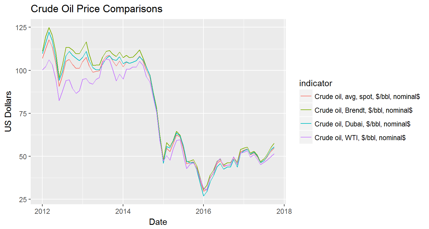

Mapping `wbstats` data with `sf`

Currently, wbstats does not include any default geometries or spatial features. However, thanks to the fantastic Simple Features R Package, we can easily add support

library(wbstats)
library(dplyr)
library(sf)

# world country polygons 'medium' scale 
world_geo <- rnaturalearth::ne_countries(scale = 50, returnclass = "sf")


pop_data <- wb(country = "countries_only", 
               indicator = "SP.POP.GROW", 
               mrv = 1)
  
pop_geo <- left_join(world_geo, pop_data, by = c("iso_a2" = "iso2c"))

Mapping with `ggplot2`

As of this writing, the version of ggplot2 on CRAN (2.2.1) does not have support for sf objects. To take advantage of the latest functionality you’ll need to download the development version of ggplot2 from github.

Matt Strimas-Mackey has a really great overview of spatial data support in the tidyverse that goes into a lot more detail on using sf objects with ggplot2, dplyr, and the rest of the tidyverse Here so I won’t go into anymore detail, but here is an example adapted from his post

library(ggplot2)
library(viridis)

ggplot(pop_geo) +
  geom_sf(aes(fill = value)) +
  scale_fill_viridis("value") +
  ggtitle("Population Growth (annual % growth)") +
  theme_bw()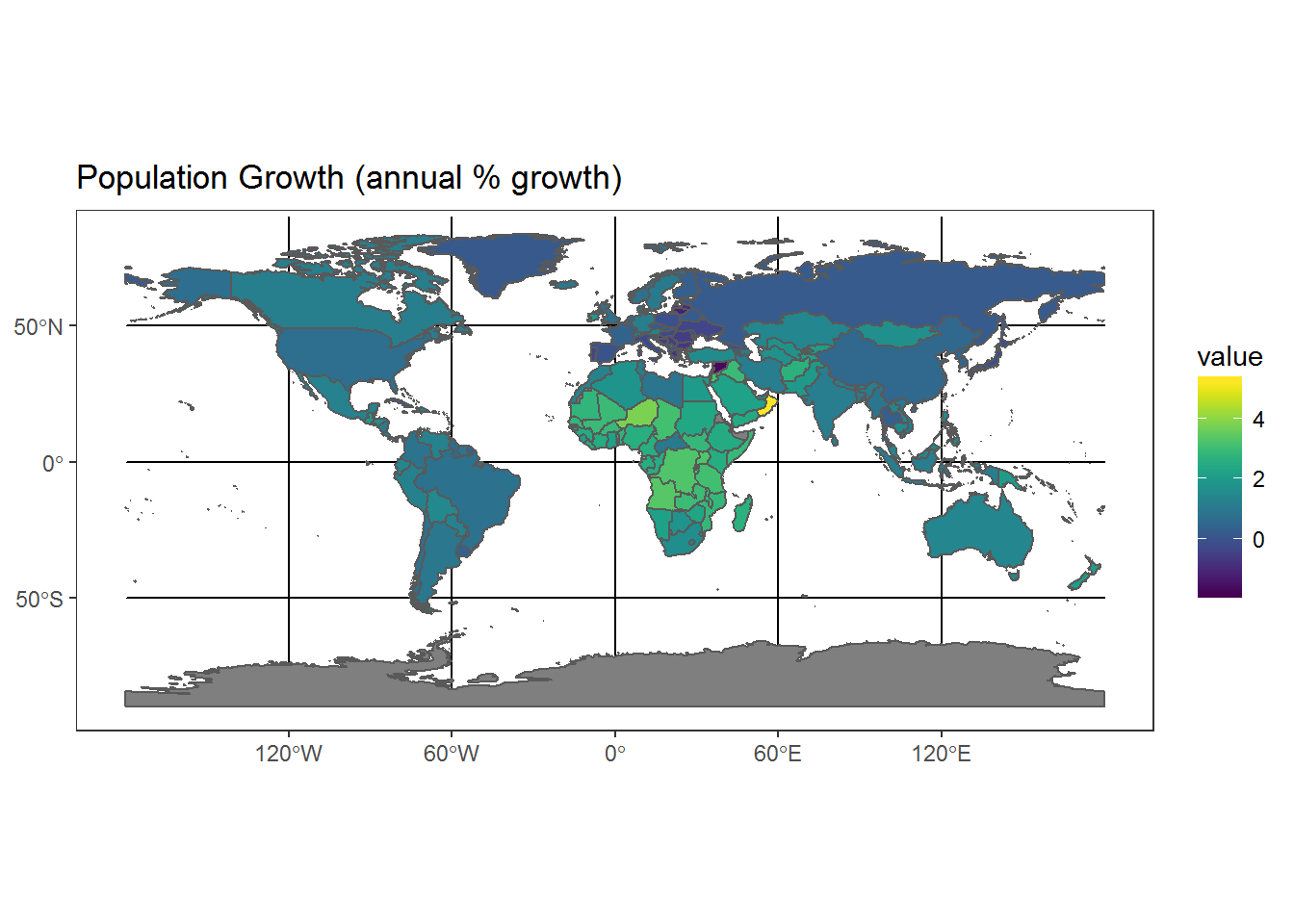

Example using `leaflet`

leaflet is a great package for online interactive maps in R. Here is the same map as above using leaflet

library(leaflet)

pal <- colorNumeric("viridis", domain = pop_geo$value)

labels <- sprintf("<strong>%s</strong><br/>%s: %g%%",
                  pop_geo$name_long, pop_geo$indicator, round(pop_geo$value, 2)) %>% 
  lapply(htmltools::HTML)

l <- leaflet(pop_geo, height = 400, width = "100%") %>%
      setView(20,25, zoom = 1) %>%
      addTiles() %>%
      addPolygons(
        fillColor = ~pal(value),
        weight = 1,
        opacity = 1,
        color = "grey",
        fillOpacity = 0.7,
        highlight = highlightOptions(
          weight = 3,
          color = "#666",
          dashArray = "",
          fillOpacity = 0.7,
          bringToFront = TRUE),
        label = labels,
        labelOptions = labelOptions(
          style = list("font-weight" = "normal", padding = "3px 6px"),
          textsize = "15px",
          direction = "auto")) %>%
      addLegend(pal = pal, values = ~value, opacity = 0.9, 
                title = NULL,
                position = "bottomright",
                labFormat = labelFormat(suffix = "%"))

l

Getting Started Indicators

Here are a few indicators that can help get you started with using the wbstats package

indicatorID	indicator
SI.POV.GINI	GINI index (World Bank estimate)
SL.UEM.TOTL.ZS	Unemployment, total (% of total labor force) (modeled ILO estimate)
SP.DYN.IMRT.IN	Mortality rate, infant (per 1,000 live births)
SP.DYN.CBRT.IN	Birth rate, crude (per 1,000 people)
SP.POP.TOTL	Population, total
SP.POP.GROW	Population growth (annual %)
NY.GDP.MKTP.KD.ZG	GDP growth (annual %)
NY.GDP.MKTP.KD	GDP (constant 2010 US$)
EN.ATM.CO2E.PC	CO2 emissions (metric tons per capita)
EN.ATM.CO2E.KT	CO2 emissions (kt)

Features Coming Soon

Full metadata search, including country, country-series, and footnotes
Better support for mapping with sf
Addition of the World Bank Projects API
Suggest a feature on Github

R wbstats

Getting Started with wbstats A World Bank R Package

Downloading data with wb

Search available data with wbsearch

One list to rule them all wb_cachelist

The countries data frame

The indicators data frame

Accessing updated available data with wbcache()

Plotting & Mapping with wbstats

Using POSIXct = TRUE

Plotting with ggplot2

Mapping wbstats data with sf

Mapping with ggplot2

Example using leaflet